Inverse Bradford Hill Criteria: How Association Flirts with Causality in Real-World Evidence, and What We Find When It Doesn’t
Drawing insights from observational data is difficult. With myriad factors influencing outcomes, establishing causality poses a daunting challenge. Association is not causality, and sometimes association is all we can get from observational data. Sometimes, conclusions based on associations contradict what we might infer through causal reasoning — (e.g. paradoxes in hospitalized patient outcomes). Every so often, though, there’s an alluring flicker, a subtle hint — association flirts with causality.

Consider the image above. It’s a representation of an individual’s change in understanding the relationship between correlation and causation — before attending a statistics class, the individual though correlation implied causation, but afterward the individual recognizes the differences. We can’t definitively state that the class caused this newfound enlightenment, but isn’t it the most plausible explanation?
Can we approach causal inference from real-world evidence? Inversely, can we discount the possibility of causality to learn about hidden confounding complex systems from associations?
Real-World Evidence: When Can Association Be Interpreted as Causal Inference?
The most useful criteria I’ve found for describing the flirtatious relationship between association and causality come from the English statistician Sir Austin Bradford Hill. In 1965, he proposed nine criteria to suggest a causal relationship between a presumed cause and an observed effect:
- Strength: The stronger the association, the more likely it is to be causal
- Consistency: The association is observed repeatedly
- Specificity: The cause leads to a specific effect
- Temporality: The cause precedes the effect
- Biological gradient (dosage effect): The effect increases with the cause
- Plausibility: The association has a plausible mechanistic explanation
- Coherence: The association is compatible with existing theory and knowledge
- Experiment: The association is confirmed by experimental evidence
- Analogy: The association is similar to other known causal relationships
Others have added to this list, most commonly “reversibility” (i.e., the effect is reversed when the cause is removed). While these criteria are not intended to be a checklist, they provide a useful framework for evaluating the strength of evidence for a causal relationship.
For the most part, these criteria are self-explanatory. Let’s look at how Mendelian Randomization applies these principles to use the natural temporality of genetics to approach causal inference from observational data.
Mendelian Randomization — The Natural Temporality of Genetics Mendelian randomization (MR) uses genetic variants as instrumental variables to estimate the causal effect of an intermediate phenotype on an outcome of interest. The main idea underlying MR is that genetic assignments temporally precede the outcome of interest, and are randomly assigned at conception, so whatever intermediate phenotype can be predicted from genetics can be interpreted as a pseudorandomly-assigned exposure. Thus, by using only the portion of the intermediate phenotype that is independent of confounding variables (i.e. the variation that is predictable from genetic variants), we can estimate causal effects influencing the outcome of interest.
To get the portion of the intermediate phenotype that is independent of confounding variables, we use instrumental variables: genetic variants that are associated with the intermediate phenotype but not associated with confounding variables. Since the genetic variants temporally preceded the outcome, and are randomly assigned at conception, they are not subject to confounding. As a result, the portion of the intermediate phenotype that is predictable from these genetic variants is also not subject to confounding.

The most common method for MR is 2-step least squares regression:
- Regress intermediate phenotype on genetic variants
- Regress outcome on intermediate phenotype
MR makes three core assumptions:
- The genetic variants are independent of the confounding variables (always false, and untestable)
- The genetic variants are strongly associated with the intermediate phenotype (testable, but often weak association)
- No other path from gene to disease outcome other than through the intermediate phenotype (always false, and untestable)
These assumptions demonstrate a bitter pill common with methods of causal inference: assumptions are often untestable, and even when they are testable, they are often false.
For this reason, it can be productive to apply tests of causality in the opposite direction: — if an association breaks the rules of causality, it’s probably not causal. This approach uncovers confounding factors, spurious associations, artifacts of real-world evidence, and opportunities to improve real-world systems.
Working Backwards: When Should Association Be Interpreted as Something Other than Causality?
By taking the inverse of the Bradford Hill criteria, we can identify situations where the association is likely to be non-causal. These could be due to confounding, spurious associations, artifacts of real-world evidence, or opportunities to improve real-world systems.
The inverse Bradford Hill criteria are:
- Weakness: The weaker the association, the less likely it is to be causal
- Inconsistency: The association is not observed repeatedly
- Non-specificity: The cause leads to multiple effects
- Non-temporality: The cause does not precede the effect
- Non-biological gradient (dosage effect): The effect does not increase smoothly with the cause
- Non-plausibility: The association does not have a plausible mechanistic explanation
- Incoherence: The association is not compatible with existing theory and knowledge
- Non-experiment: The association is not confirmed by experimental evidence
- Non-analogy: The association is not similar to other known causal relationships
- Irreversibility: The effect is not reversed when the cause is removed
Let’s consider a few of these in more detail.
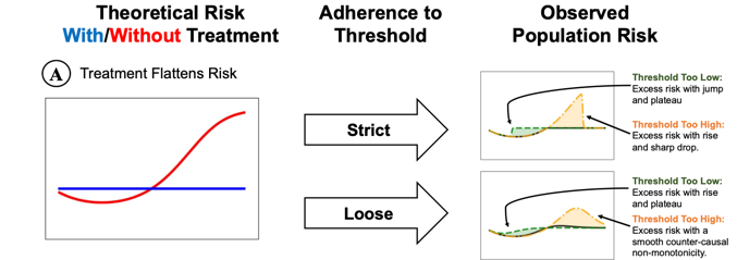
Non-Biological Gradients (Discontinuities and Non-Monotonicities) According to the Bradford Hill criteria, greater exposure should generally lead to greater incidence of the effect. In other words, there should be a biological gradient, or dosage effect. In real-world evidence with data arising from human systems, we often see discontinuities and non-monotonicities instead of smooth gradients. These discontinuities and non-monotonicities are often an indication of confounding from systemic processes like treatment decisions.
For example, in the care of hospitalized patients, there may be a decision of whether or not a patient is given a particular treatment. There is often a threshold for this decision, such that patients above the threshold are more likely to receive the treatment, ideally set where the risk of the treatment is outweighed by the benefit. However, if the threshold is off, we may see a characteristic pattern in the association between the biomarker and the outcome at the threshold. The pattern is either a sharp discontinuity if the adherence to the treatment threshold is strict, or a smooth non-monotonicity if adherence to the treatment threshold is loose.

This evidence of systemic confounding is strengthened when these non-biological gradients occur at round-number thresholds. For example, in the context of hospitalized patient outcomes, we often see jumps in mortality at round-number ages, which is likely due to the fact that patients are treated differently at round-number ages (e.g., 65, 70, 75, 80, etc.).
Non-plausibility
According to the Bradford Hill criteria, causal associations should have a plausible mechanistic explanation. In real-world evidence, we often see associations that are not biologically plausible, which is a strong indication that the association is not causal. For example, consider the following example from the ICU: elevated creatinine levels indicate acute kidney injury (AKI), which would be expected to be linked to increased mortality. But in real-world evidence, elevated creatinine levels are associated with decreased mortality. Applying the inverse Bradford Hill criteria, this association is not biologically plausible, and therefore not likely to be causal. Prompted by this finding of non-causal association, we may look for confounding factors in treatment decisions that explain this non-causal association (in fact, ICU patients with AKI are more likely to be given dialysis and/or renal replacement therapy, which is associated with improved mortality). Importantly, because this association is not causal, it can likely be fixed by improving the real-world system of healthcare.
Incoherence
According to the Bradford Hill criteria, the association should be compatible with existing theory and knowledge. With the rise of foundation models such as large language models (LLMs), we can now check this criterion automatically. For example, we can check the above example of AKI and mortality by asking an LLM whether the graph of mortality vs creatinine makes sense in light of the LLM’s prior knowledge.
The package TalkToEBM makes this simple:
import t2ebm
gpt4 = guidance.llms.OpenAI("gpt-4")
ebm = ExplainableBoostingClassifier(feature_names=feature_names)
ebm.fit(X_train, y_train)
graph_desc = t2ebm.llm_describe_ebm_graph(gpt4, ebm, 0) # 0 is the feature index
The output of TalkToEBM on the creatinine example is:

Complications of Causality in Practice: Do We Really Want Causal Models?

In practice, we often want models that are not causal. Consider sepsis prediction, in which we’d like to build a system to alert clinicians when patients are at high risk of developing sepsis, so that they could be treated. The most accurate predictive models contain variables such as prior antibiotic usage which are influenced by the clinician’s concern about sepsis risk. This is not a biologically causal variable, but it is a useful variable for predicting sepsis risk.
In this case, we may want to build a model that is not causal, but is instead a good predictor of sepsis risk. Such a predictive model may not be good for making decisions about sepsis treatment (e.g., for many patients, antibiotic prescription may be a large contribution to the predicted risk of sepsis, intervening by taking away antibiotics would be exactly the wrong action but could be recommended by derivative-based analyses of the predictive model). On the other hand, building a causal model of sepsis may not produce accurate predictions of sepsis risk, and therefore may not be useful for alerting clinicians to patients at high risk of sepsis.
It’s critical to carefully describe the exact use case of the model we are designing — biologically causal models may not be the most useful model.
Conclusion
Causal inference is a powerful tool for understanding the world, but it is not a panacea, especially in observational data. In this post, we’ve discussed the Bradford Hill criteria, which are a set of rules for determining whether an association is likely to be causal.
In practice, it can be more productive to use the inverse Bradford Hill criteria to determine an association is likely to be non-causal. When an association is non-causal, it may be due to confounding, spurious associations, artifacts of real-world evidence, or opportunities to improve real-world systems. We’ve discussed several examples of non-causal associations, and how they can be used to improve real-world systems like creatinine monitoring in the ICU. Finally, we’ve discussed the complications of causality in practice, and how causal models may not be the best models for many real-world use cases.


